Data Preprocess

Including methods implemented during EDA and data lacking.

Lack of Training Data (数据短缺)

---

Data Augmentation (数据增强)

Expand an input dataset by slightly changing the existing (original) examples. (e.g.: crop, rotate, zoom, flip and color the input images)

Transfer Learning (迁移学习)

Synthetic Data (合成数据)

Feature Aggregation/Engineering (特征聚合/工程)

Combine features to form new features. (e.g.: Combine ‘length’ and ‘width’ to form ‘area’)

Feature Transformation (特征转换)

Discretization (离散化)

Turn numerical data into categorical. (e.g.: Turn ‘Age’ into <20, >=20, <25 and >=25)

EDA: Exploratory Data Analysis (探索性数据分析)

---

Summary Statistics (总结统计量)

Measures of Location for continuous features

1. Mean: 均值
2. Median: 中位数
3. Mode: 众数
4. Quantiles: 分位数

Measures of Spread for continuous features

1. Range: minimum and maximum
2. Variance: ‘how far’ values are from ‘mean’
3. Standard Deviation
4. Interquartile ranges(IQR)

Data Cleaning (数据清洗)

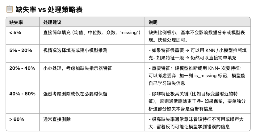
Missing Values

There may be some missing values in the training/test set. We should find and handle them properly.

# If there is any missing values?

df.isnull().values.any()

# see how many missing values there are in each feature(column).

missing_values = df.isnull().sum()  # return a Series, indicating each column
missing_values = missing_values[missing_values > 0]   # return columns which have missing values 

Deletion

Straightforward, but can be problematic if a big portion of data is missing.

Mean/Median/Mode Imputation

# Show information of pandas df, and see if there is any 'Nan' values
dataframe.info()

# Fill by SimpleImputer
from sklearn.impute import SimpleImputer

# by 'mean' value
imputer = SimpleImputer(strategy='mean')

# by 'most_fequent' value
imputer = SimpleImputer(strategy='most_frequent')

# by 'median' value
imputer = SimpleImputer(strategy='median')

dataframe['column_name'] = imputer.fit_transform(dataframe['column_name'])  # Reminder: if this column is object dtype, may should add '.flatten()' at the end

K-Nearest Neighbors Imputation (KNN)

Used as a predictive performance benchmark when you are trying to develop more sophisticated models.

Hyperparameters in KNN: 1. ‘K’, 2. Distance Metrics, 3. Weighting Scheme: Uniform, Distance based and Custom Weights
Weighted KNN: Give more weight to the nearby points and less weight to the far away points.
Pros and Cons: Easy to understand and lazy learning. Usually works well when the number of dimensions is small but things fall apart quickly as goes up

Model-based Imputation

Interpolation (插值法)

Estimate the value of missing values based on the surrounding trends and patterns. This approach is ‘more feasible’ to use when your ‘missing values are not scattered too much’.

1. Random under-sampling: Randomly eliminating the samples from the majority class until the classes are balanced in the remaining dataset (Cut the major class to less).
2. Random over-sampling: Instances of the minority class by random replication of the already present samples (Better than over-sampling).
3. Synthetic over-sampling (SMOTE: 合成过采样): A subset of minority class is taken, and new synthetic data points are generated based on it.

)

Outliers

Detect and remove lines which contain outliers using IQR.

from scipy.stats import iqr

Q1 = df.quantile(0.25)
Q3 = df.quantile(0.75)
IQR = Q3 - Q1

df_without_outliers = df[~((df < Q1 - 1.5 * IQR) | (df > Q3 + 1.5 * IQR)).any(axis=1)]

Feature Scaling (特征放缩)

Normalization (归一化)

In normalization, you are changing the distribution of your data into ‘normal distribution’.

Use this when you’re going to use a ML or statistics technique that assumes your data is normally distributed.
Use in neural networks, KNN, K-means.
Scale feature to a fixed range: [0, 1] or [-1, -1].

For feature $X$,
$$
X_{normalized} = \frac{X\ -\ X_{min}}{X_{max} - X_{min}}
$$

Standardization (标准化)

In standardization, it will assume that your raw data displays a normal distribution and scale data to distribute as a standard normal distribution with mean = 0 and standard deviation = 1.
For feature $X$,
$$
X_{standardized} = \frac{X\ -\ \mu}{\sigma},\ where\ \mu\ is\ mean\ of\ X,\ \sigma\ is\ standard\ deviation\ of\ X
$$

Some models or algorithms (linear/logistic regression, SVM, PCA) are sensitive to data distribution, use Standardization to make standard normal distribution.

Feature Encoding (特征编码)

Label Encoding

Suitable for nominal data with no order.

One-Hot Encoding

For the features contain limited numbers of string classes(e.g. gender: female and male, embarked class: S, C and Q) and the categories have no ranking, use One-Hot Encoding to encode.

from sklearn.preprocessing import OneHotEncoder

encoder = OneHotEncoder()
df['column_name'] = encoder.fit_transform(df['column_name'])

Ordinal Encoding

Preserves the order of ordinal data.

Target Encoding

Effective when there’s a relationship between the categorical feature and the target variable.

Frequency Encoding

Useful for handling high-cardinality features.

Feature Selection (特征选择)

Remove features which aren’t relevant to the task. (e.g.: patientID to the health status)

Heatmap + PCA

• Use heatmap to check correlations between all features.
• If there are some features that have high correlation(say > 0.8) with each other (this is called: Multi-collinearity(多重共线性)), but all have low correlation(say < 0.2) to target. This means they are redundant features.
• Use PCA to decrease dimension and remove redundant features.

Dimensionality Reduction (特征降维)

Among all your features, there are many features that 1.have low correlation with the target label, 2.have high correlation between each other(multicollinearity). That’s why we need dimensional reduction.

---

PCA (principle component analysis 主成分分析)

Reduces dimensionality by maximizing variance. It is unsupervised and works with the data as a whole, without considering class labels.

Implement PCA

1. Standardization
2. Calculate covariance matrix
3. Calculate eigenvalues and eigenvectors (特征值和特征向量)
4. Sort eigenvalues and their corresponding eigenvectors
5. Pick k eigenvalues and form a matrix of eigenvectors
6. Transform the original matrix

Pros and Cons

1. PCA works only if the observed variables are linearly correlated.
2. Will loss information.
3. Helps to remove noise and less important features that have low variance.
4. Reveals the underlying structure and relationships in the data, useful for pattern discovery.

LDA (linear discriminant analysis 线性判别分析)

Reduces dimensionality by maximizing class separability. It is supervised and uses class labels to find directions that separate the classes.

1. Primarily utilized in supervised classification problems.
2. LDA assumes:
   a. data has a normal distribution
   b. the covariance matrices of the different classes are equal
   c. the data is linearly separable

LDA Criteria

1. Maximize the distance between the means of the two classes.
2. Minimize the variation within each class.

Pros and Cons

1. Ideal when the goal is to separate classes as efficiently as possible.
2. Suitable for small to medium datasets with fewer features, effective for problems with more than two classes.
3. Could handle multicollinearity and combine correlated features efficiently.

t-SNE (t-Distributed Stochastic Neighbor Embedding)

Data Splitting (数据分割)

Train/Validation/Test Split

Training Dataset: The sample of data used to fit the model.
Validation Dataset: The sample of data used to provide an unbiased evaluation of a model fit on the training dataset while tuning model hyperparameters.
Test Dataset: The sample of data used to provide an unbiased evaluation of a final model fit on the training dataset.

Only using a portion of your data for training and only a portion for validation. If your dataset is small you might end up with a tiny training and/or validation set.

Cross-Validation

Split the data into k folds (often k=10). Each “fold” gets a turn at being the validation set.