
Logistic Regression (逻辑回归模型)
logistic regression model~
Logistic Regression
Compared with linear regression, logistic regression is used to solve questions which only have limited possible answers.
For example, if an email is spam or not, if a tumour is malignant or benign and so on. Logistic regression predicts discrete values.
Sigmoid Function
For classification problems, we also starts by using the linear regression model, $f_{\vec{w},b}(\vec{x}) = \vec{w} \cdot \vec{x} + b$ .
However, we would like the predictions of our classification model to be between 0 and 1 since our output variable 𝑦 is either 0 or 1.
So here we’re introducing “sigmoid function“ which maps all input values to values between 0 and 1.
$$
sigmoid: g(z) = \frac{1}{1 + e^{-z}}
$$
Logistic Regression
A logistic regression model applies the sigmoid to the familiar linear regression model:
$$
f_{w,b}(\mathbf{x}^{(i)}) = g(\mathbf{w} \cdot \mathbf{x}^{(i)} + b)
$$
where
$$
g(z) = \frac{1}{1 + e^{-z}}
$$
Decision Boundary
We now know the answers of classification problems are discrete, and logistic regression models predict values range from 0 to 1 after using sigmoid function.
But how do we get the final predict, like a tumour is malignant or benign? We can’t give a predict like, ‘this tumor has 75% chance to be benign’. It must be a certain answer.
So, we need to make decision boundary.
Assume that ‘y = 1’ represents the positive result, like ‘benign’, and ‘y = 0’ refers to the negative result, ‘malignant’. We can use a threshold = 0.5 to split the values of the model as below:
if $f_{w,b}(x) >= 0.5$ , y = 1
if $f_{w,b}(x) < 0.5$ , y = 0
According to the logistic regression description above,
$f_{w,b}(x) = 0.5$ means $g(z) = 0.5$, then we can get the value of $z$.
The function $z = \mathbf{w} \cdot \mathbf{x} + b$ is just the decision boundary under a threshold of 0.5.
Cost Function
When we implement the cost function of linear regression to logistic regression, it turns out to be a non-convex function and not suitable for logistic regression.
So we are using a new function called ‘Logistic Loss Function’.
Loss Function
Loss is a measure of the difference of a single example to its target value.
Cost is a measure of the losses over the entire training set.
For a single data point: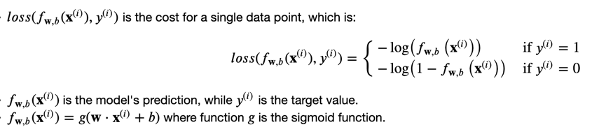
Cost Function
To form the cost function, we combine the losses.
$$
J(w, b) = \frac{1}{m} \sum_{i=0}^{m-1} \left[ loss(f_{w,b}(\mathbf{x}^{(i)}), y^{(i)}) \right]
$$
Gradient Descent in Logistic Regression
Logistic regression uses almost the same pattern as linear regression, except the function “f”.
$$
\frac{\partial}{\partial w} J(w, b) = \frac{1}{m} \sum_{i=1}^{m} \left( f^{(i)} - y^{(i)} \right) x^{(i)}
$$
$$
\frac{\partial}{\partial b} J(w, b) = \frac{1}{m} \sum_{i=1}^{m} \left( f^{(i)} - y^{(i)} \right)
$$
where $ f = g(z) = sigmoid(z), z = \vec{w} \cdot \vec{x} + b $
Summary
From this lesson, we now learn a new regression model called ‘Logistic Regression’ and how to implement gradient descent on it. It’s used to solve classification problems.
We also learn a method called ‘Regularization’ and add the regularization term to cost function for both linear and logistic regression, in order to solve overfitting problem.